Use Cases
This section of the DIVA Framework documentation will work users through typical use cases that they are likely to encounter as they work on DIVA releated tasks.
Working with DIVA Data Sets
The first DIVA task you’ll likely want to accomplish is to examine the DIVA data, particulary the provided annotations. The DIVA framework provides a number of tools that facilitate this. This section will discuss how to use them.
Simple Annotations
The central processing mechanism is the Sprokit pipeline. Pipelines are dynamically configurable using .pipe files that allow the connection of a number of procressing nodes to accomplish a specific task. In this case, we’ll create a pipeline that reads a video file and set of annotaitons, draws teh annottaion bounding boxes on the images and makes them available for review.
To do this, you’ll need to build the DIVA framework. You’ll also need the pipeline_runner command which should be in your PATH if you source <diva framework build directory>/setup_DIVA.sh after you’ve built the DIVA framework.
A .pipe file that will accomplish this task can be found at view_diva_annotations.pipe. To familiarize you with the use of pipelines and to introduce some of the basic capabilities of the DIVA framework we’ll examine that pipeline file in detail here.
The first element in the pipeline opens and reads the video data:
process input
:: video_input
video_filename      = /Users/kfieldho/Projects/Kitware/Vision/Data/DIVA/V1/VIRAT_S_000000.mp4
frame_time         = .3333
video_reader:type  = vidl_ffmpeg
What this says is that we’re creating a process in our pipeline called input which is of type video_input. We set a number of configuration parameters for this process the most important of which is the video_filename which should provide the full path name of the video file you want to visualize.
We’ll create another process that reads the appropriate annotations. The DIVA program provides annotations in two formats. The first is a JSON format that is used by NIST as they run their evalautions. The second is a KPF format used as a native format with the KWIVER framework on which DIVA framework is based which in some cases carries more information than the JSON format which may be useful. For now we will concern ourselves with the KPF format:
process annotations
  :: detected_object_input
  file_name = /Users/kfieldho/Projects/Kitware/Vision/Data/DIVA/V1/VIRAT_S_000000.geom.yml
  reader:type = kpf_input
We’re creating a detected_object_input process called annoations. The reader:type configuration parameter tells Sprokit to load the kpf_input implementation of detected_object_input. Perhaps the most important configuration parameter is file_name which specifies the input file. In this case we’re going to use the “geom” KPF file provided with the DIVA dataset corresponding with the video that we’ve selected. (KPF is storage agnostic, YAML is used for the delivery of KPF files related to the DIVA program). The “geom” file carries the bounding boxes for the annotations, which we’ll be visualizing with the next section of the .pipe file:
process draw_annotations
  :: draw_detected_object_set
  :draw_algo:type ocv
  :draw_algo:ocv:default_color 0 250 0
  :draw_algo:ocv:default_line_thickness 2
  :draw_algo:ocv:draw_text false

connect from input.image to draw_annotations.image
connect from annotations.detected_object_set to draw_annotations.detected_object_set
Here’re we’re creating a draw_detected_object_set process called draw_annotations. To configure this process, we’ll explore further some of the capabilities of the Sprokit/KWIVER pipeline system. First, we’ll introduce a new command plugin_explorer that will help us learn about the plugins available in the system. First, we’ll get the documenation for draw_detected_object_set by issuing the command plugin_explorer –process draw_detected_object_set –detail:
Process type: draw_detected_object_set
Description:       Draws border around detected objects in the set using the selected
    algorithm.

    This process is a wrapper around a draw_detected_object_set algorithm.

  Properties: _no_reentrant

  -- Configuration --
  Name       : draw_algo
  Default    :
  Description:       Name of drawing algorithm config block./n/nSpecify an implementation of
    the draw_detected_object_set algorithm as draw_algo:type = <type>
  Tunable    : no

-- Input ports --
  Name       : detected_object_set
  Data type  : kwiver:detected_object_set
  Flags      : _required
  Description: Set of detected objects.

  Name       : image
  Data type  : kwiver:image
  Flags      : _required
  Description: Single frame image.

-- Output ports --
  Name       : image
  Data type  : kwiver:image
  Flags      :
  Description: Single frame image.
First, this output tells us that there’s a configuration setting called draw_algo that should specify an implemenation of draw_detected_object_set as draw_algo:type. We’ll use plugin_explorer to learn more about these algorithms by issueing the command plugin_explorer –algorithm draw_detected_object_set –detail:
Plugins that implement type "draw_detected_object_set"
---------------------
Info on algorithm type "draw_detected_object_set" implementation "ocv"
  Plugin name: ocv
      Draw bounding box around detected objects on supplied image.
    -- Configuration --
    "alpha_blend_prob" = "true"
    Description:       If true, those who are less likely will be more transparent.

    "clip_box_to_image" = "false"
    Description:       If this option is set to true, the bounding box is clipped to the image
      bounds.

    "custom_class_color" = ""
    Description:       List of class/thickness/color seperated by semicolon. For example:
      person/3/255 0 0;car/2/0 255 0. Color is in RGB.

    "default_color" = "0 0 255"
    Description:       The default color for a class (RGB).

    "default_line_thickness" = "1"
    Description:       The default line thickness, in pixels.

    "draw_text" = "true"
    Description:       If this option is set to true, the class name is drawn next to the
      detection.

    "select_classes" = "*ALL*"
    Description:       List of classes to display, separated by a semicolon. For example:
      person;car;clam

    "text_scale" = "0.4"
    Description:       Scaling for the text label. Font scale factor that is multiplied by the
      font-specific base size.

    "text_thickness" = "1"
    Description:       Thickness of the lines used to draw a text.

    "threshold" = "-1"
    Description:       min threshold for output (float). Detections with confidence values below
      this value are not drawn.
In this case there is only one algorithm plugin, ocv that applies. The output provides the list of configuration options that we can select. In the example pipeline, we choose to set default_color, default_line_thickness and draw_text.
At this point, we’ve defined most of the processes we need in our pipeline. Now we must connect them together in order for the pipeline to accomplish something. Looking back at the process documentation for draw_detected_object_set we see a listing of the input ports for the process, specifically an image port and a detected_object_set. We can use plugin_explorer to examine the detected_object_input process to see that it has an output port of detected_object_set. Given this we can use the connect command in the pipeline to connect the detected_object_set output port of detected_object_input to the detected_object_set input port of draw_detected_object_set. Similarly, we can connect the image output port of the video_input process to the image input port of draw_detected_object_set.
Finally, we’ll want to see the result of the annotated images. We’ll create an image_writer process and connect the image output of the draw_detected_object_set process to its corresponding image input port. We configure the image_writer to write its output to the OUTPUT directory in our current working directory, naming each image with an “image” prefix and a zero padded frame number. by using the “.jpg” extension, we will get JPEG output images. We could have used “.png” for PNG images.
Running the pipeline is straightforward:
pipeline_runner --pipeline view_diva_annotations.pipe
We can then review the resulting images with our favorite image viewer:
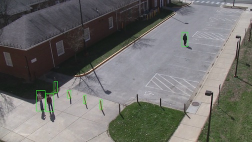
Simple Frame Annotation of DIVA Data Set
Integrating an Activity Detector
To create a pluggable modules that the DIVA framework can detect/use during deployment, you will
use the Sprokit process interface. This ensures consistency in the data flow, allowing
different process nodes to interact with each other. An algorithm can be expressed
as a single process or a pipeline of processes based on developer’s requirements. Currently,
the DIVA framework supports Python and C++ processes that are created by inheriting
KWIVERProcess and sprokit::process respectively. Implementing the process interface
can be divided into three components:
Defining Ports: The data flow amongst processes is managed using
ports. The inputportsindicate input for the algorithm. Similarly, the outputportsindicate the output of the algorithm. For example, the DIVA baseline algorithmRC3DDetectordeclaresimage,timestampandfile_nameas input ports anddetected_object_setas its only output port. Theseportsuse `Vital types <complex data types_>`_ to transmit complex data structures designed for vision based applications. Additionally, if these types do not cover an algorithms input/output requirement, additional Vital types can be created. Refer to the tutorial on `Extending Vital Types`_ for additional information.Adding Configuration Parameters: `Configuration parameter <config_>`_ are used to specify algorithm parameters. These parameters are declared by a process and can be specified when the process is added to a pipeline or at runtime. In addition to traditional configuration parameters, processes frequently make use of KWIVER’s
AbstractAlgorithmcapability to allow a configuration parameter to select among several implementations of the processes algorithm. Refer to the tutorial on Tight Integration and `Extending KWIVER`_ for details.Overriding
_configureand_stepfunctions: The_configurefunction is called process instantiation and is responsible for retrieving and applying configuration parameters. The_stepfunction is called for each processing step (typically for each frame of video input) and retrieves data from the process input ports, manipulates and transforms that data in some way and puts the resulting data on its output port for processing by down stream nodes in the pipeline.
For more details about sprokit processes, refer to Processes.
The data flow amongst the modules is defined as a `pipeline`_ (actually a directed acyclic graph of processing nodes). The pipeline declares the process present, provides configuration parameters for every process and connects the ports for the process. The framework supports expressing pipelines using plain text file or programmatically in Python or C++. Refer to Pipelines for more additional information.
To execute a plain text pipeline file, the DIVA framework uses an executable
provided by KWIVER, pipeline_runner. The executable accepts a .pipe file
as input along with any configuration parameter adjustments and runs the pipeline:
pipeline_runner -p test.pipe --set test_process:configuration_name=test
The usage information for pipeline_runner is documented in detail here.